Chapter 1: Introduction to Short Time Fourier Transform

The Short Time Fourier Transform (STFT) is a pivotal technique in time-frequency analysis, particularly useful for observing how certain frequencies change over time. This methodology is especially beneficial when analyzing signals that vary dynamically.

To implement the STFT, the process begins by dividing the time-domain signal into smaller segments using a sliding window approach. Each segment undergoes a Fourier transformation, allowing for detailed frequency analysis within specified time frames.

For practical application, you would typically start by importing essential libraries and creating a simulated dataset. The following code snippet demonstrates this:

import numpy as np

import matplotlib.pyplot as plt

from scipy.signal import stft

Imagine you're conducting an experiment and gathering time series data. It's crucial to consider several factors during data collection:

• Total number of samples (N)
• Sampling rate (the number of samples collected per unit time, usually in seconds, denoted as n)

For example:

N = 600 # Number of sample points

Fs = 800.0 # Sampling frequency (samples per second)

T = 1.0 / Fs # Sample period; duration of each sample

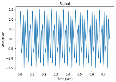
Next, a hypothetical dataset can be generated based on these parameters, representing a linear combination of two sinusoidal waves at 50 Hz and 80 Hz:

x = np.linspace(0.0, N*T, N)

y = np.sin(50.0 * 2.0 * np.pi * x) + 0.5 * np.sin(80.0 * 2.0 * np.pi * x)

To perform the STFT, we'll utilize the stft() function from the scipy library. The parameters required for this function include:

• y: The time series data
• Fs: The sampling frequency
• window: The window function for slicing (details will be provided later)
• padded: A boolean indicating whether to apply zero-padding on each slice

When the stft() function is applied to the time series array, it returns:

• fft[0]: An array of sample frequencies
• fft[1]: An array of segment times
• fft[2]: The STFT of the input array

Here’s how to execute it:

fft = stft(y, Fs, window='hann', padded=True)

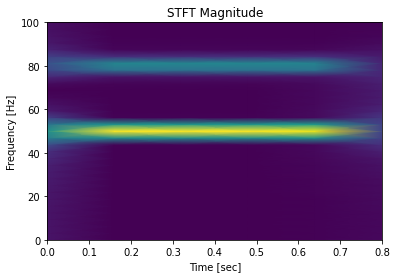
For visualization, we can create a time-frequency analysis plot:

plt.pcolormesh(fft[1], fft[0], np.abs(fft[2]), shading='gouraud')

plt.title('STFT Magnitude')

plt.ylabel('Frequency [Hz]')

plt.xlabel('Time [sec]')

As observed, the temporal changes in sample frequencies are displayed. Notably, the intensity of both frequencies tends to remain fairly stable, with slight variations at the beginning and end due to the slicing of the raw data.

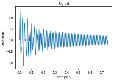
Next, let's introduce an exponential damping factor to the pseudo-data, which will create interesting variations over time for the respective frequencies:

y_damp = (np.sin(50.0 * 2.0 * np.pi * t) * np.exp(-t / 0.1)) + (0.5 * np.sin(80.0 * 2.0 * np.pi * t) * np.exp(-t / 0.8))

Now, the signal visualization will appear as follows:

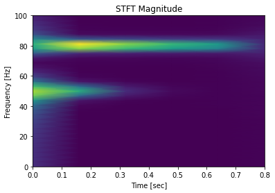
Repeating the steps under the same conditions will yield a new time-frequency analysis map:

In this analysis, the two frequencies are observed to change over time while adhering to their distinct decay rates (0.1 seconds for 50 Hz and 0.8 seconds for 80 Hz).

For further insights, stay tuned for upcoming discussions on this topic. Happy reading!

If you're interested in deeper exploration, consider subscribing to the membership program for full access to all stories on Medium! Trust me, you won't regret it!

Chapter 2: Video Insights on STFT

Explore the mechanics of the Short Time Fourier Transform (STFT) in this video, which outlines its application in time-frequency analysis.

In this video, the Short-Time Fourier Transform is explained in a straightforward manner, making it easier to grasp its significance in signal processing.