Exploring Chaos in Classical Mechanics: The Double Pendulum
Written on
Understanding Classical Mechanics
Classical mechanics focuses on the motion of objects influenced by forces. This field, which has been studied for centuries, remains essential in physics and serves as a basis for various disciplines. A key concept in classical mechanics is the equations of motion, which help forecast the behavior of objects and systems over time.
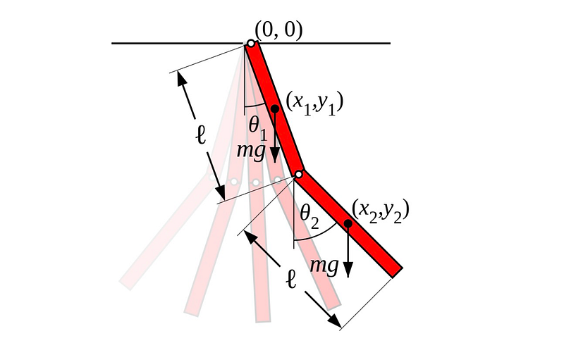
The double pendulum is a prime illustration of a system characterized by intricate motion governed by classical mechanics. This setup comprises two pendulums connected to one another, where the motion of one pendulum impacts the other. Notably, the double pendulum displays chaotic dynamics, where minor variations in initial conditions can result in dramatically divergent paths over time.
In this article, we will derive the equations of motion for the double pendulum using Lagrange mechanics and implement the solution using Python's odeint function. Following that, we will visualize the pendulum's animated motion to observe its chaotic behavior.

Lagrange Mechanics and Motion Equations
To establish the equations of motion, we utilize Lagrange mechanics. As outlined in “God’s Own Equation Solved with Python,” the Lagrangian needs to be expressed in chosen coordinates. The Lagrangian, defined as kinetic energy minus potential energy, is given by:

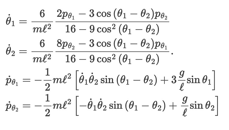
By applying the Euler-Lagrange equations to this Lagrangian, we derive the equations of motion:

Here, the p’s represent the conjugate momenta of ?1 and ?2, respectively.
To facilitate calculations, we organize the independent variables into a vector y:

Thus, our equations can be expressed in a standard form that is compatible with most ordinary differential equation solvers:

The following Python function defines the right-hand side of our equations:
def f(y, t):
dy0_dt = 6./(m*L**2) * (2 * y[2] - 3 * np.cos(y[0]-y[1]) * y[3])/(16 - 9 * np.cos(y[0]-y[1])**2)
dy1_dt = 6./(m*L**2) * (8 * y[3] - 3 * np.cos(y[0]-y[1]) * y[2])/(16 - 9 * np.cos(y[0]-y[1])**2)
dy2_dt = -.5 * m * L**2 * ( dy0_dt * dy1_dt * np.sin(y[0]-y[1]) + 3 * (g/L) * np.sin(y[0]))
dy3_dt = -.5 * m * L**2 * (-dy0_dt * dy1_dt * np.sin(y[0]-y[1]) + (g/L) * np.sin(y[1]))
return [dy0_dt, dy1_dt, dy2_dt, dy3_dt]
We can compute the system's equations utilizing Python's odeint function from the scipy.integrate library. Initially, we define the function f(y, t), which accepts the vector of independent variables y and time t as inputs and returns the derivative of y concerning t. Subsequently, we establish the initial conditions y_init, time points t, and call odeint. The result is an array y, which holds the values of y at each time point. The motion of the double pendulum can be visualized using matplotlib, allowing us to examine its chaotic behavior over time:
import numpy as np
from scipy.integrate import odeint
y_init = [np.pi / 2.75, np.pi / 2, 0, 0]
t = np.linspace(0, 50, 2000)
y = odeint(f, y_init, t)
import matplotlib.pyplot as plt
fig, ax = plt.subplots()
ax.plot(t, y[:, 0], label=r"$theta_1$")
ax.plot(t, y[:, 1], label=r"$theta_2$")
ax.set_xlabel("time (s)")
ax.set_ylabel("angle (radians)")
ax.legend()

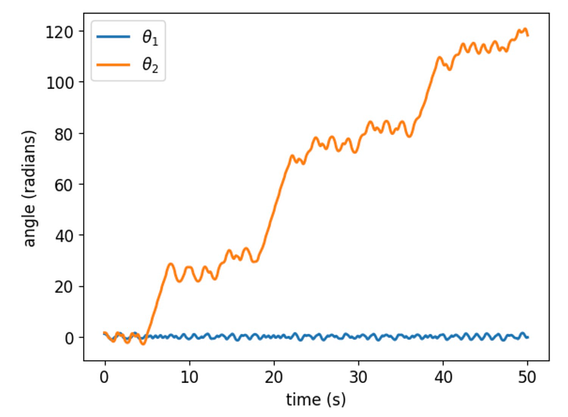
The motion of the double pendulum can be categorized into two phases. Initially, the movement resembles oscillation, with the pendulums swaying back and forth. However, after a brief period, the second pendulum flips, leading to increasingly unpredictable and non-repetitive motion. This chaotic behavior indicates that even slight alterations in the initial conditions can cause substantial variations in trajectories over time. The underlying non-linear interactions between the two pendulums give rise to this chaotic behavior, which is prevalent in many physical systems and has significant implications in areas such as weather forecasting and stock market analysis.
Animating the Double Pendulum
We can create an animation of the double pendulum's motion using matplotlib's animation capabilities:
from matplotlib import animation
%matplotlib notebook
fig, ax = plt.subplots(figsize=(5,5))
ax.set_xlim([1, -1])
ax.set_ylim([-1.5, 0.5])
plt.axis("off")
dt = t[1] - t[0]
pendulum_1, = ax.plot([], [], "r")
pendulum_2, = ax.plot([], [], "b")
def init():
pendulum_1.set_data([], [])
pendulum_2.set_data([], [])
def animate(frame):
ax.set_title("Time: %10.2f s" % (frame * dt))
x_1 = L * np.sin(y[frame, 0])
y_1 = - L * np.cos(y[frame, 0])
x_2 = x_1 + L * np.sin(y[frame, 1])
y_2 = y_1 - L * np.cos(y[frame, 1])
pendulum_1.set_data([0, x_1], [0, y_1])
pendulum_2.set_data([x_1, x_2], [y_1, y_2])
return [pendulum_1, pendulum_2]
anim = animation.FuncAnimation(fig, animate, frames=len(t), interval=20)

After approximately five seconds, the second pendulum experiences several flips. The animate function updates the pendulums' positions at each time step, while the FuncAnimation class constructs an animation from these updates. Observing the double pendulum's chaotic behavior reveals the complexity introduced by the system's non-linear dynamics, where minor changes in initial conditions can lead to drastic differences in trajectories. The double pendulum serves as one of the simplest chaotic systems in classical mechanics, highlighting the significance of understanding non-linear system behaviors.
Conclusion
In summary, the double-compound pendulum presents an intriguing system that demonstrates chaotic behavior within classical mechanics. We derived the motion equations using Lagrange mechanics and solved them with Python's odeint function. By visualizing the motion of the double pendulum through matplotlib, we witnessed the complex and unpredictable behavior arising from the system's non-linear dynamics.